Analysis of single cell RNA-Seq data using scTernary

Introduction

Ternary plot is a good method to visualize three-dimensional data. scTernary is an easy and user friendly package to show three different single cell populations as well as the potential intermediate cell populations on the ternary plot. The ternary plot method can also be utilized to investigate cell lineage segregation.

Installation

The scTernary package can be installed from GitHub by using:

devtools::install_github("jinming-cheng/scTernary")

Ternary plot analysis for 10x single cell RNA-Seq data

Load package

library(scTernary)

Obtain raw count matrix from an example Seurat object containing cells from adult mouse mammary gland epithelium.

data_exp_mat <- example_seu@assays$RNA@counts
data_exp_mat <- as.matrix(data_exp_mat)
#> Loading required package: Matrix
dim(data_exp_mat)
#> [1] 13750    80

Mouse signature genes for Basal, LP and ML cells

head(anno_signature_genes_mouse)
#>        GeneID        Symbol Chr gene_type
#> 497097 497097          Xkr4   1     Basal
#> 329093 329093          Cpa6   1     Basal
#> 320492 320492 A830018L16Rik   1     Basal
#> 240725 240725         Sulf1   1     Basal
#> 14048   14048          Eya1   1     Basal
#> 226866 226866        Sbspon   1     Basal

Number of signature genes for each cell type

table(anno_signature_genes_mouse$gene_type)
#> 
#> Basal    LP    ML 
#>  1470   428   529

Prepare data for ternary plot. A constant raw count cut-off of 0 is used to count the number of genes for each signature gene type.

data_for_ternary <- generate_data_for_ternary(
  data_exp_mat = data_exp_mat,
  anno_signature_genes = anno_signature_genes_mouse,
  gene_name_col = "Symbol",
  gene_type_col = "gene_type",
  weight_by_gene_count = TRUE,
  cutoff_exp = 0,
  prior_count = 1
)

head(data_for_ternary)
#>                             Basal         LP         ML
#> Adult-CGGAGGCTGTCTGA-1 0.06108202 0.03217158 0.01113586
#> Adult-ATCTCAACGAACCT-1 0.13263525 0.04825737 0.03563474
#> Adult-TGGAAGCTTACAGC-1 0.09773124 0.05361930 0.02449889
#> Adult-CTTCTAGACTGTGA-1 0.07329843 0.03753351 0.02672606
#> Adult-AAGACAGATTGGTG-1 0.06806283 0.02949062 0.01336303
#> Adult-TTGAGGACGTTTGG-1 0.06806283 0.08579088 0.01559020

Add metadata to the data for ternary plot

data_for_ternary <- cbind(data_for_ternary,example_seu@meta.data)

Draw the ternary plot colored by cell type. Mouse mammary gland epithelium contains three major cell types: Basal, LP and ML. In this example, an additional luminal intermediate cell population can be easily observed by using the ternary plot method.

scTernary::vcdTernaryPlot(data_for_ternary,
                          order_colnames=c(2,3,1),
                          point_size = 0.5,
                          group = data_for_ternary$cell_type_label,
                          show_legend = TRUE,
                          scale_legend = 0.8,
                          legend_position = c(0.3,0.5),
                          legend_vertical_space = 1,
                          legend_text_size = 1)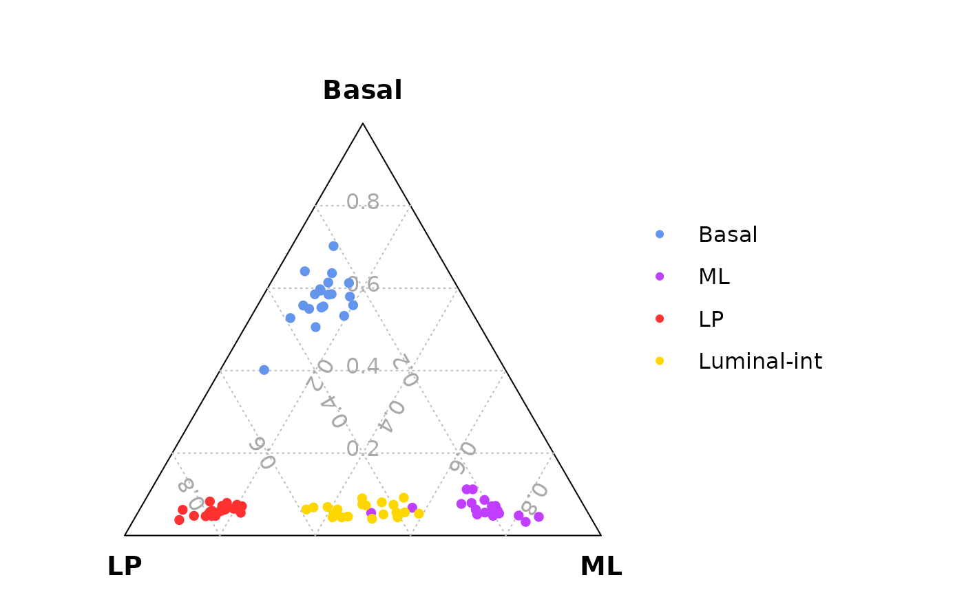

Ternary plot analysis for exploring cell lineage segregation

The public 10x scRNA-seq data of mouse mammary epithelial cells at different stages reanalyzed by Cheng et al. 2023. F1000Res. can be used to investigate cell lineage segregation or commitment. The ternary plot analysis suggests that the lineages of mammary epithelial cells are segregated at post-natal 5 days (P5).

Load data for ternary plot from Cheng et al generated by using generate_data_for_ternary function

load(system.file("extdata", "data_for_ternary_Cheng.rda",package = "scTernary"))
head(data_for_ternary_Cheng)
#>                                    Basal         LP         ML     group
#> GSM4994960-AAACCTGAGAGACTTA-1 0.15256688 0.12068966 0.07053942 E18.5-epi
#> GSM4994960-AAACCTGCAAACGCGA-1 0.11424440 0.09605911 0.09128631 E18.5-epi
#> GSM4994960-AAACCTGCACAGCCCA-1 0.17787419 0.18719212 0.11410788 E18.5-epi
#> GSM4994960-AAACCTGGTAGCGTGA-1 0.11352133 0.05665025 0.04149378 E18.5-epi
#> GSM4994960-AAACCTGGTGAAAGAG-1 0.06869125 0.03694581 0.04356846 E18.5-epi
#> GSM4994960-AAACCTGTCAAGGTAA-1 0.08026030 0.06403941 0.03526971 E18.5-epi

Mouse mammary epithelial cells at 5 different stages

table(data_for_ternary_Cheng$group)
#> 
#>   E18.5-epi          P5 Pre-puberty     Puberty       Adult 
#>        4343        1140        2546        4706        9341

Ternary plots of mouse mammary epithelium samples at five different stages. The results demonstrate that mammary epithelial cell lineages are not segregated at embryonic 18.5 days (E18.5), and the cells are segregated at post-natal 5 days (P5) but not well differentiated. At pre-puberty stage the cells are completely segregated and almost well differentiated, and there are many luminal-intermediate cells. At puberty and adult stages, the three cell lineages are clear, and there are fewer luminal-intermediate cells than pre-puberty stage.

# An example of setting figure width and height
n_col = 3
n_row = 2
n_scale_legend = 2
fig_width = 2*n_col + 1*n_scale_legend
fig_height = 2*n_row

# png(filename = "TernaryPlot.png",width = fig_width,height = fig_height,units = "in",res = 300)
vcdTernaryPlot(data = data_for_ternary_Cheng,
  order_colnames = c(2,3,1),
  group = data_for_ternary_Cheng$group,
  facet = TRUE,
  point_size = 0.2,
  show_legend = TRUE,
  legend_point_size = 0.6,
  legend_position = c(0.4,0.5),
  scale_legend = n_scale_legend)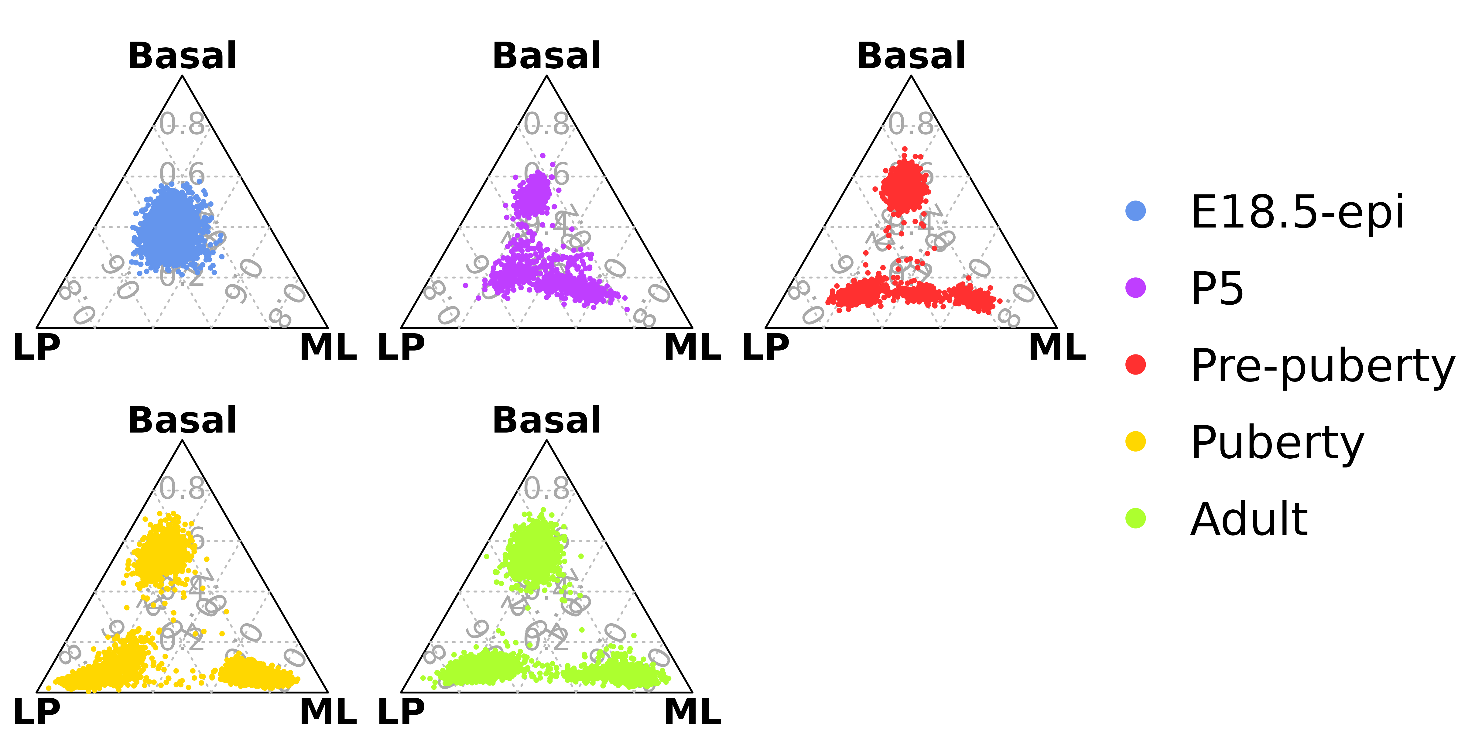

# dev.off()

Ternary plot analysis for Fluidigm C1 data or bulk RNA-Seq data

Ternary plot analysis using a constant cut-off

The number of genes and library size of Fluidigm C1 single cell RNA-Seq data is quite similar to bulk RNA-Seq data. Hence, we use a small bulk RNA-Seq dataset to show the ternary plot analysis for Fluidigm C1 data.

Example bulk RNA-seq data (using CPM)

cpm <- edgeR::cpm(example_dge_data$counts)

Three samples for each group

example_dge_data$samples$group
#> [1] LP    ML    Basal Basal ML    LP    Basal ML    LP   
#> Levels: Basal LP ML

Generate data for ternary plot using a CPM cut-off of 100

data_for_ternary <- generate_data_for_ternary(
  data_exp_mat = cpm,
  anno_signature_genes = anno_signature_genes_mouse,
  gene_name_col = "GeneID",
  gene_type_col = "gene_type",
  weight_by_gene_count = TRUE,
  cutoff_exp = 100,
  prior_count = 2
)

head(data_for_ternary)
#>                Basal         LP         ML
#> 10_6_5_11 0.02244898 0.34579439 0.07750473
#> 9_6_5_11  0.02040816 0.16822430 0.29300567
#> purep53   0.21020408 0.06074766 0.03402647
#> JMS8-2    0.21496599 0.05841121 0.03591682
#> JMS8-3    0.02380952 0.21495327 0.26654064
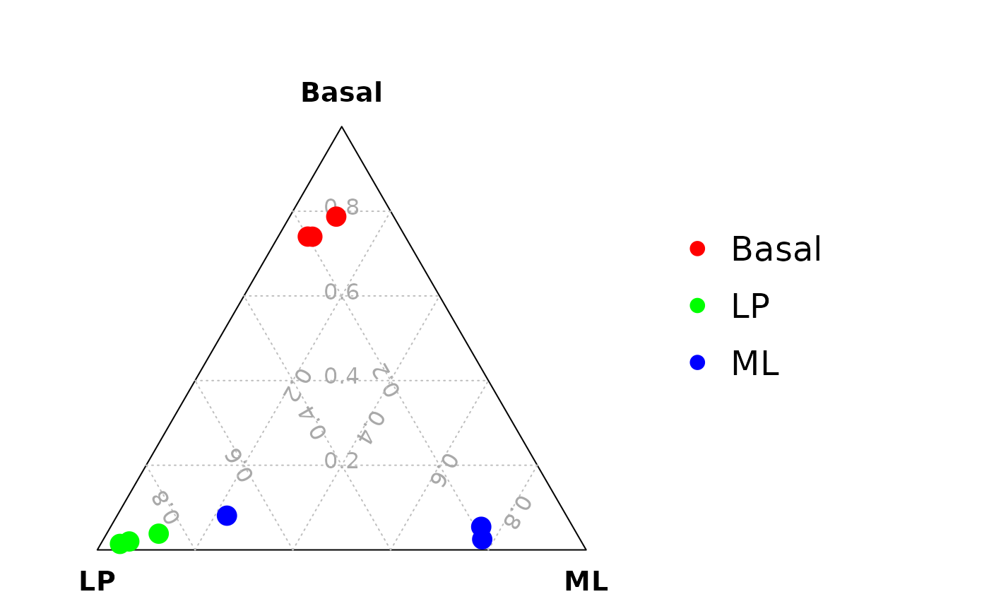
#> JMS8-4    0.02040816 0.33878505 0.09451796

Drawing the ternary plot

vcdTernaryPlot(data = data_for_ternary,
  order_colnames = c(2,3,1),
  group = example_dge_data$samples$group,
  group_color = c("red","green","blue"),
  point_size = 1,
  show_legend = TRUE,
  legend_point_size = 0.6,
  legend_position = c(0.3,0.5),
  scale_legend = 1)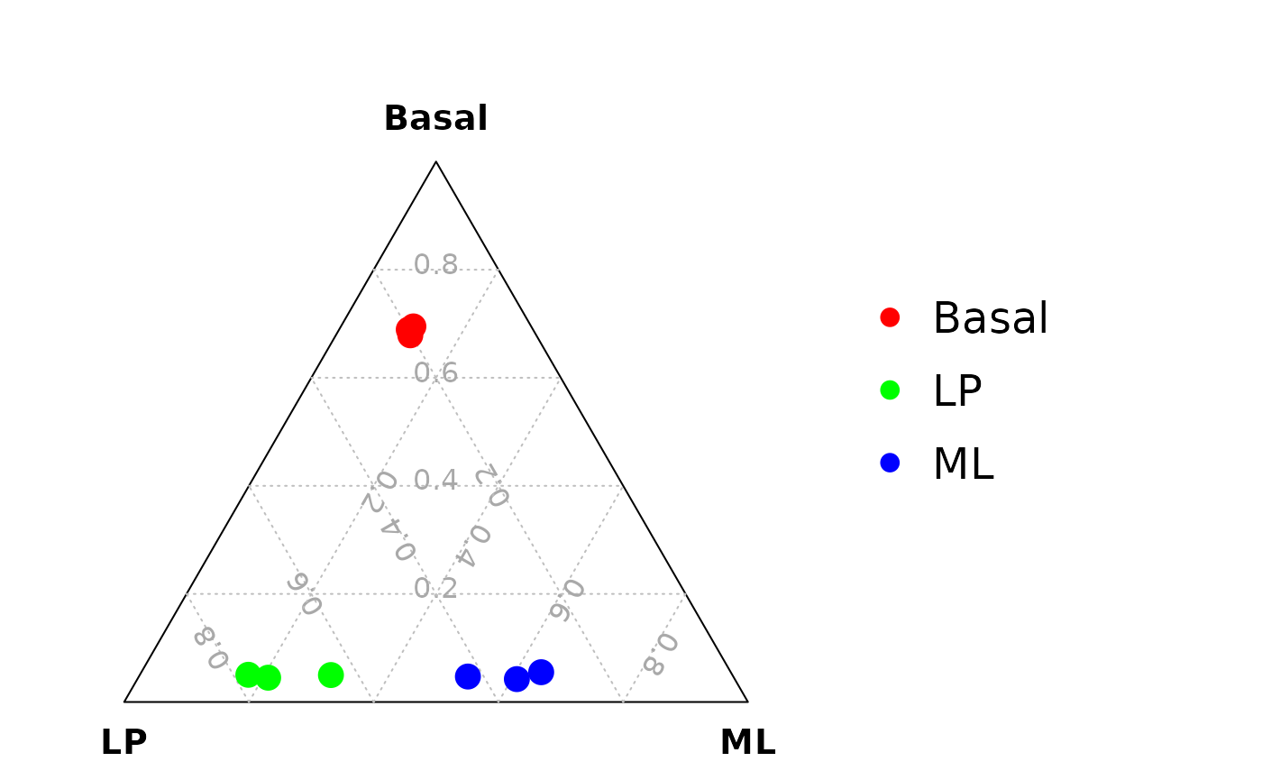

Ternary plot analysis using estimated cut-offs

We can also find the optimized cut-off for each sample (or cell) to calculate the signature gene proportion for the sample (or cell). The optimized cut-off is estimated by maximizing the coefficient of variation (CV) of the signature gene proportion by a grid search method.

Example bulk RNA-seq data (using logCPM)

lcpm <- edgeR::cpm(example_dge_data$counts,log = TRUE)

Three samples for each group

example_dge_data$samples$group
#> [1] LP    ML    Basal Basal ML    LP    Basal ML    LP   
#> Levels: Basal LP ML

Estimate a optimized cut-off for each sample (or cell)

estimated_cutoffs <- estimate_optimized_cutoffs(
  data_exp_mat = lcpm,
  anno_signature_genes = anno_signature_genes_mouse,
  gene_name_col = "GeneID",
  gene_type_col = "gene_type",
  weight_by_gene_count = TRUE,
  prior_count = 2,
  do_parallel = TRUE,
  n_cores = 2
)

Generate data for ternary plot

data_for_ternary <- generate_data_for_ternary(
  data_exp_mat = lcpm,
  anno_signature_genes = anno_signature_genes_mouse,
  gene_name_col = "GeneID",
  gene_type_col = "gene_type",
  weight_by_gene_count = TRUE,
  cutoff_exp = estimated_cutoffs,
  prior_count = 2
)

head(data_for_ternary)
#>                 Basal          LP          ML
#> 10_6_5_11 0.001360544 0.091121495 0.003780718
#> 9_6_5_11  0.001360544 0.004672897 0.018903592
#> purep53   0.100000000 0.025700935 0.009451796
#> JMS8-2    0.031292517 0.004672897 0.003780718
#> JMS8-3    0.001360544 0.011682243 0.003780718
#> JMS8-4    0.001360544 0.063084112 0.003780718