Getting Started with SpNeigh

Introduction

Recent spatial transcriptomics technologies such as 10x Xenium, MERFISH, and Visium HD enable high-resolution profiling of gene expression while preserving tissue architecture. These platforms have opened new avenues for studying tissue organization, cell–cell interactions, and spatial gene regulation.

Most existing methods focus on identifying globally spatially variable genes or enhancing spatial visualization, with limited support for modeling local spatial context, such as region boundaries, cell neighborhoods, or gradients across tissue structures.

SpNeigh is an R package that introduces a boundary-aware and region-informed framework for spatial neighborhood analysis and spatial differential expression modeling. Key features include:

Boundary detection and neighborhood ring construction
Spatial weighting using distances to centroids or boundaries
Spline-based modeling of gene expression along spatial gradients
A spatial enrichment index (SEI) to quantify boundary- or region-enriched genes

Unlike existing Bioconductor tools such as spatialDE, which emphasize global spatial variability, SpNeigh enables local, interpretable, and geometry-aware modeling of spatial expression patterns.

SpNeigh supports inputs from both SpatialExperiment and Seurat objects for coordinate extraction and visualization, and emphasizes transparent modeling using user-supplied matrices and weights—ensuring reproducibility and compatibility with Bioconductor workflows.

By integrating spatial geometry with transcriptomic data, SpNeigh reveals biologically meaningful patterns such as intermediate cell states, microenvironmental differences, and spatial gene expression gradients, which are critical for understanding development, tissue function, and disease progression.

Overview of this vignette

This vignette demonstrates the key functionalities of the SpNeigh package using a real
10x Xenium Fresh Frozen Mouse Brain Tiny Subset dataset.

Specifically, we show how to:

Identify spatial boundaries and construct neighboring ring regions
Explore spatial interaction patterns between cell clusters
Perform differential expression analysis between spatially defined cell populations
Compute spatial weights based on boundary or centroid proximity
Model spatial expression gradients using spline-based differential expression
Quantify spatial enrichment along spatial gradients

This workflow highlights the analytical flexibility of SpNeigh and illustrates how neighborhood-aware modeling can reveal spatial gene expression patterns that are not readily captured by existing approaches.

Installation

The SpNeigh package can be installed from GitHub by using:

devtools::install_github("jinming-cheng/SpNeigh")

Load packages

library(SpNeigh)
library(ggplot2)

Load data

Input: Coordinate data frame and Normalized expression matrix

Coordinates of mouse brain dataset

coords <- readRDS(system.file("extdata", "MouseBrainCoords.rds",
    package = "SpNeigh"
))
head(coords)
#>          x        y cell cluster
#> 1 1898.815 2540.963    1       4
#> 2 1895.305 2532.627    2       4
#> 3 2368.073 2534.409    3       2
#> 4 1903.726 2560.010    4       4
#> 5 1917.481 2543.132    5       4
#> 6 1926.540 2560.044    6       4

Ensure the rownames of coords are the same with the cell names

rownames(coords) <- coords$cell

Log normalized expression data generated by NormalizeData function in Seurat package

logNorm_expr <- readRDS(system.file("extdata", "LogNormExpr.rds",
    package = "SpNeigh"
))
class(logNorm_expr)
#> [1] "dgCMatrix"
#> attr(,"package")
#> [1] "Matrix"

Annotate clusters based on anatomical brain regions

new_cell_types <- c(
    "0" = "Meninges",
    "1" = "Cerebral_cortex",
    "2" = "White_matter",
    "3" = "Cerebral_cortex",
    "4" = "Cerebral_cortex",
    "5" = "Thalamus",
    "6" = "Cerebral_cortex",
    "7" = "Hippocampus",
    "8" = "Hippocampus",
    "9" = "Hippocampus",
    "10" = "White_matter",
    "11" = "Cerebral_cortex"
)

In this vignette, we focus on cluster-level rather than cell type–level analyses.

Alternative input: SpatialExperiment object

Coordinates of cells in clusters 0 and 2

coords_sub <- subset(coords, cluster %in% c("0", "2"))
coords_sub <- as.matrix(coords_sub[, c("x", "y")])

metadata of cells in clusters 0 and 2

metadata_sub <- subset(coords[, c("cell", "cluster")], cluster %in% c("0", "2"))

Create SpatialExperiment

spe <- SpatialExperiment::SpatialExperiment(
    assay = list("logcounts" = logNorm_expr),
    colData = metadata_sub,
    spatialCoords = coords_sub
)
spe
#> class: SpatialExperiment 
#> dim: 248 11617 
#> metadata(0):
#> assays(1): logcounts
#> rownames(248): 2010300C02Rik Acsbg1 ... Zfp536 Zfpm2
#> rowData names(0):
#> colnames(11617): 3 8 ... 36595 36597
#> colData names(3): cell cluster sample_id
#> reducedDimNames(0):
#> mainExpName: NULL
#> altExpNames(0):
#> spatialCoords names(2) : x y
#> imgData names(0):

Extract coordinates from SpatialExperiment object

spe_coords <- extractCoords(spe)

Extract log-normalized expression matrix from SpatialExperiment object

spe_logcounts <- SingleCellExperiment::logcounts(spe)

Alternative input: Seurat object

Load Seurat pacakge

library(Seurat)
#> Loading required package: SeuratObject
#> Loading required package: sp
#> 'SeuratObject' was built with package 'Matrix' 1.7.1 but the current
#> version is 1.7.4; it is recomended that you reinstall 'SeuratObject' as
#> the ABI for 'Matrix' may have changed
#> 
#> Attaching package: 'SeuratObject'
#> The following objects are masked from 'package:base':
#> 
#>     intersect, t

Create Seurat object (Note: a normalized expression matrix is used here for tutorial purposes only. In practice, use a raw count matrix.)

seu_sp <- CreateSeuratObject(
    assay = "Spatial",
    counts = logNorm_expr,
    meta.data = metadata_sub
)
seu_sp
#> An object of class Seurat 
#> 248 features across 11617 samples within 1 assay 
#> Active assay: Spatial (248 features, 0 variable features)
#>  1 layer present: counts

Insert normalized data into the data layer (Seurat v5)

LayerData(seu_sp, assay = "Spatial", layer = "data") <- logNorm_expr

Add FOV

cents <- CreateCentroids(coords_sub[, c("x", "y")])

fov <- CreateFOV(
    coords = list("centroids" = cents),
    type = c("centroids"),
    assay = "Spatial"
)

seu_sp[["fov"]] <- fov

Add seurat_clusters to the metadata

seu_sp$seurat_clusters <- seu_sp$cluster

Extract coordinates from Seurat object

seu_sp_coords <- extractCoords(seu_sp)

Extract log-normalized expression matrix from Seurat object

seu_sp_log_expr <- GetAssayData(seu_sp)

Neighborhood analysis for cluster 2 cells

Quick look at the boundaries of one cluster

Quick look at the boundaries of cluster 2 using default parameter settings. The input is a SpatialExperiment object.

plotBoundary(spe, one_cluster = "2")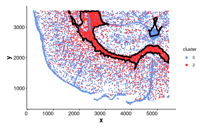

Similarly, we can use a Seurat object as input and adjust parameters

plotBoundary(seu_sp, one_cluster = "2", eps = 120)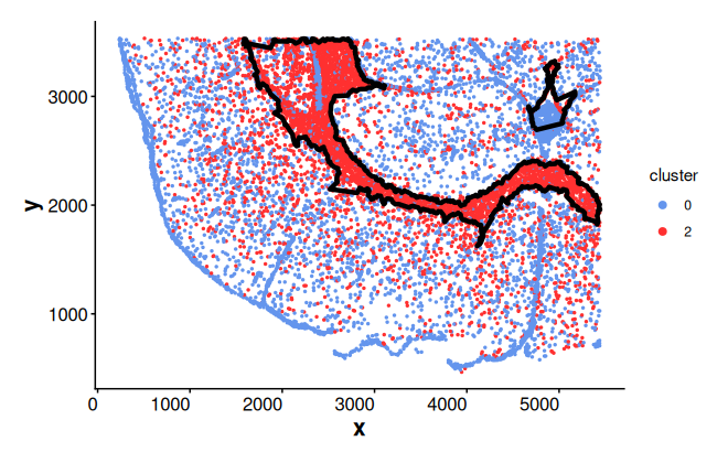

Detect spatial boundaries

Extract boundaries of cluster 2. Adjust the eps and minPts parameters to refine the number of subregions detected by the default dbscan clustering method.

Note: The eps parameter controls the clustering tolerance for boundary detection based on spatial distance. The default value is eps = 80, which is suitable for coordinates in the range of hundreds or thousands (e.g., 10x Xenium or Visium HD data). For datasets with smaller coordinate ranges (e.g., 1 to 5), such as manually scaled or normalized inputs, a smaller value such as eps = 0.1 may be more appropriate.

bon_points_c2 <- getBoundary(
    data = coords,
    one_cluster = 2,
    eps = 120,
    minPts = 10
)
table(bon_points_c2$region_id)
#> 
#>   1   2 
#> 572 132

Add boundaries of cluster 2 to the spatial plot

plotBoundary(coords, boundary = bon_points_c2)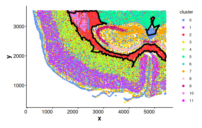

Alternatively, add boundaries of cluster 2 using addBoundary() function

# plotBoundary(coords) + addBoundary(boundary = bon_points_c2)

Plot boundary regions

bon_polys_c2 <- buildBoundaryPoly(bon_points_c2)
plotRegion(bon_polys_c2)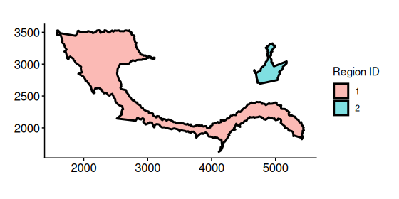

Obtain neighborhood ring regions

Get spatial ring-shaped regions by subtracting the original boundary polygons from their corresponding outer buffered polygons. The outer_boundary is automatically computed when it is not supplied.

ring_regions <- getRingRegion(boundary = bon_points_c2)

Plot ring regions

plotRegion(ring_regions)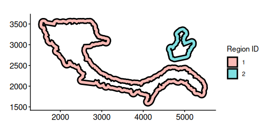

Statistics of cells inside rings

Get cells inside rings for cluster 2. (getCellsInside() takes a few seconds to run on this example, but may require several minutes or longer for larger datasets.)

cells_ring <- getCellsInside(data = coords, boundary = ring_regions)
cells_ring
#> Simple feature collection with 4362 features and 3 fields
#> Geometry type: POINT
#> Dimension:     XY
#> Bounding box:  xmin: 1482.997 ymin: 1530.545 xmax: 5441.679 ymax: 3532.463
#> CRS:           NA
#> First 10 features:
#>    cell cluster region_id                  geometry
#> 21   21       4         1 POINT (2080.017 2559.984)
#> 22   22       4         1 POINT (2088.025 2526.528)
#> 23   23       2         1 POINT (2085.119 2546.843)
#> 24   24       2         1 POINT (2101.906 2549.501)
#> 25   25       4         1 POINT (2102.112 2540.185)
#> 26   26       4         1 POINT (2089.812 2539.796)
#> 27   27       4         1  POINT (2095.253 2533.08)
#> 28   28       4         1  POINT (2100.02 2527.252)
#> 29   29       4         1 POINT (2197.507 2524.511)
#> 30   30       3         1 POINT (2209.931 2542.314)

Plot cells inside rings

plotCellsInside(cells_ring, point_size = 0.2)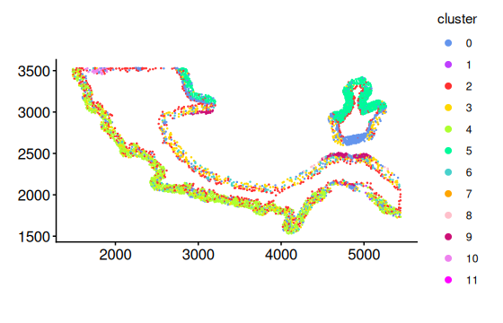

Obtain statistics of cells inside rings for cluster 2

stats_ring <- statsCellsInside(cells_ring)

Plot proportion of cells in different clusters for each sub region using bar plot.

plotStatsBar(stats_ring, stat_column = "proportion")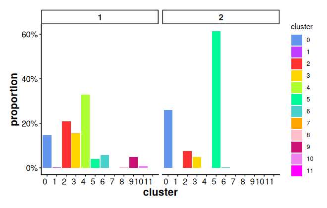

Plot proportion of cells in different clusters for each sub region using donut chart. If plot_donut = FALSE, pie chart is used.

plotStatsPie(stats_ring, plot_donut = TRUE)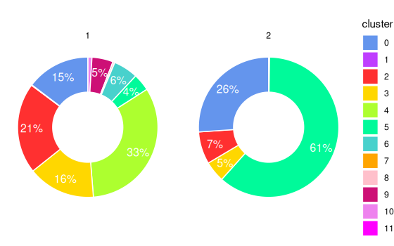

Neighborhood interaction of clusters inside rings

Compute neighborhood interaction matrix using K-nearest neighbors for cells inside rings

interaction_matrix <- computeSpatialInteractionMatrix(
    subset(coords, cell %in% cells_ring$cell)
)
interaction_matrix
#>       0  1    2    3    4    5   6 7  8    9  10 11
#> 0  4090  6 1020  892  882  706 202 6 15   95  46  0
#> 1     6  0   10   10   11    0   3 0  0    0   0  0
#> 2  1266 10 1831 1127 1882  648 392 2  0   49  72  1
#> 3   980  8  973 1409 1190  104 422 3 28  187  13  3
#> 4   859  3 1685 1185 5684    0 392 0  0    0   0  2
#> 5   768  0  501   91    0 8227  10 0  0    3   0  0
#> 6   199  1  331  442  411   12 193 0 14   99   6  2
#> 7     7  0    3    9    0    0   0 0  0    1   0  0
#> 8    20  0    5   43    0    0  20 0 29   13   0  0
#> 9   108  0   39  158    0    1  79 0 11 1064   0  0
#> 10   43  0   64   12    1    0   5 0  0    0 155  0
#> 11    0  0    1    3    4    0   2 0  0    0   0  0

Heatmap of a row-scaled interaction matrix for cells inside rings for cluster 2. The heatmap reveals that clusters 2, 3, and 4 are spatially adjacent to one another.

plotInteractionMatrix(interaction_matrix)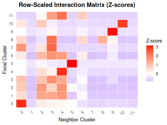

The plot of cells inside rings split by clusters further confirms the co-occurrence of clusters 2, 3, 4 in ring region 1.

plotCellsInside(cells_ring) +
    facet_wrap(~cluster) +
    Seurat::RotatedAxis() +
    addBoundaryPoly(ring_regions, linewidth_boundary = 0.1)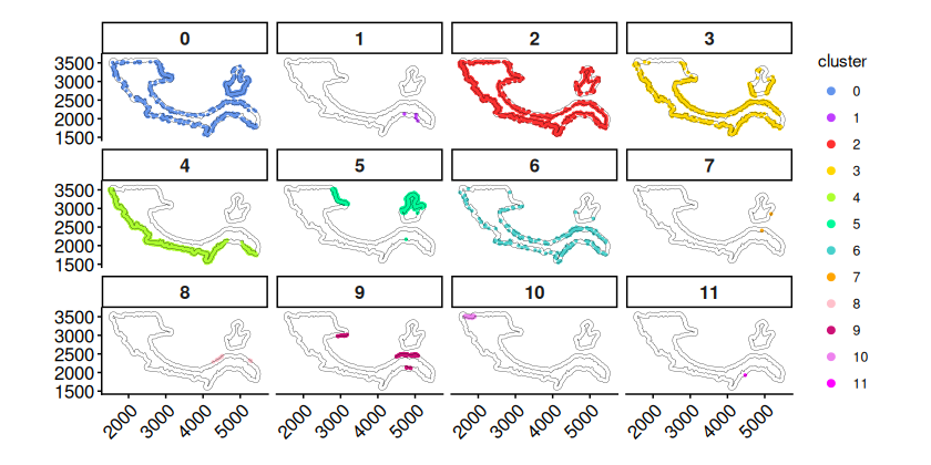

DE analysis of cluster 2 cells inside and outside boundaries

Most cells in cluster 2 are located in sub region 1. Hence, we focus on the DE analysis between cluster 2 cells inside boundary of sub region 1 and cells in the outside neighboring ring region 1.

Get cells inside the boundaries of cluster 2

cells_inside <- getCellsInside(data = coords, boundary = bon_points_c2)
cells_inside
#> Simple feature collection with 5073 features and 3 fields
#> Geometry type: POINT
#> Dimension:     XY
#> Bounding box:  xmin: 1590.613 ymin: 1640.136 xmax: 5443.607 ymax: 3531.379
#> CRS:           NA
#> First 10 features:
#>    cell cluster region_id                  geometry
#> 3     3       2         1 POINT (2368.073 2534.409)
#> 20   20       2         1 POINT (2456.959 2560.494)
#> 31   31       2         1 POINT (2152.998 2554.538)
#> 43   43       2         1 POINT (2312.183 2555.867)
#> 44   44       2         1  POINT (2323.21 2551.805)
#> 50   50       2         1 POINT (2356.391 2544.839)
#> 52   52       2         1 POINT (2387.844 2537.827)
#> 53   53       2         1 POINT (2401.216 2526.458)
#> 54   54       2         1 POINT (2392.535 2555.696)
#> 55   55       2         1 POINT (2407.538 2545.443)

Obtain cluster 2 cells inside and outside boundary of sub region

cells_in <- subset(cells_inside, region_id == 1 & cluster == 2)[["cell"]]
cells_out <- subset(cells_ring, region_id == 1 & cluster == 2)[["cell"]]

Perform DE analysis between cells inside boundary and outside boundary using the limma framewrok (lmFit + eBayes)

tab <- runLimmaDE(
    exp_mat = logNorm_expr,
    min.pct = 0.25,
    cells_reference = cells_in,
    cells_target = cells_out
)

Top DE genes between cells outside boundary and cells inside boundary. The DE genes are ordered by the abstract value of logFC by default.

head(tab[, c("gene", "logFC", "adj.P.Val", "pct.reference", "pct.target")])
#>            gene    logFC     adj.P.Val pct.reference pct.target
#> Slc17a7 Slc17a7 2.719412 1.624032e-145     0.3228372  0.7555911
#> Cabp7     Cabp7 2.256859 1.316819e-126     0.2325064  0.6453674
#> Arc         Arc 1.932350  7.188753e-73     0.4567430  0.7779553
#> Neurod6 Neurod6 1.788980 5.267216e-123     0.1224555  0.5063898
#> Igfbp4   Igfbp4 1.608183  8.429609e-96     0.1437659  0.4952077
#> Nrn1       Nrn1 1.590518  4.942213e-65     0.2722646  0.5926518

Set a random seed to make plotExpression results reproducible

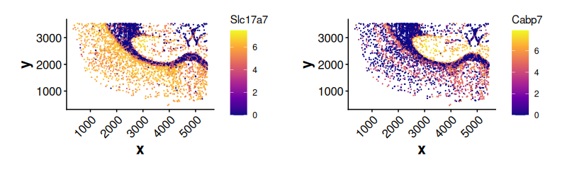
set.seed(123)

Expression of top DE genes in cluster 2 cells outside boundary. The cells are plotted randomly using the given seed when shuffle = TRUE. If shuffle = FALSE, cells with higher expression values are plotted last (on the top).

plotExpression(
    data = coords[colnames(logNorm_expr), ],
    exp_mat = logNorm_expr,
    genes = tab$gene[1:2],
    sub_plot = TRUE,
    one_cluster = 2,
    shuffle = TRUE,
    point_size = 0.1,
    angle_x_label = 45
)

Expression of Slc17a7 for cluster 2 cells inside and outside boundary of sub region 1. Cluster 2 cells outside the boundary show much higher expression of Slc17a7.

plotExpression(
    data = coords[colnames(logNorm_expr), ],
    exp_mat = logNorm_expr,
    genes = "Slc17a7",
    sub_plot = TRUE,
    shuffle = TRUE,
    sub_cells = c(cells_in, cells_out),
    point_size = 0.3
) +
    addBoundaryPoly(bon_polys_c2[1, ], linewidth_boundary = 0.5)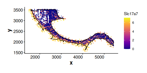

Expression of a general marker gene Sox10 for Oligodendrocytes (cluster 2 cells). Sox10 is expressed in both cluster 2 cells inside and outside the boundary. This suggests that cluster 2 cells located near the boundary may represent intermediate cell states.

plotExpression(
    data = coords[colnames(logNorm_expr), ],
    exp_mat = logNorm_expr,
    sub_cells = c(cells_in, cells_out),
    sub_plot = TRUE,
    genes = "Sox10",
    shuffle = TRUE,
    point_size = 0.3
) +
    addBoundaryPoly(bon_polys_c2[1, ], linewidth_boundary = 0.5)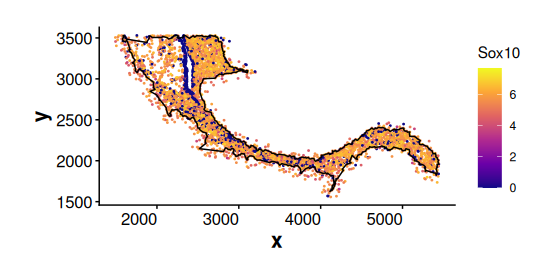

Spatial DE analysis of cells in cluster 0 along spatial weights

Detect spatial boundaries

Obtain cells in cluster 0

cells_c0 <- subset(coords, cluster == 0)[, "cell"]

Plot cluster 0 cells without boundary

plotBoundary(coords[cells_c0, ])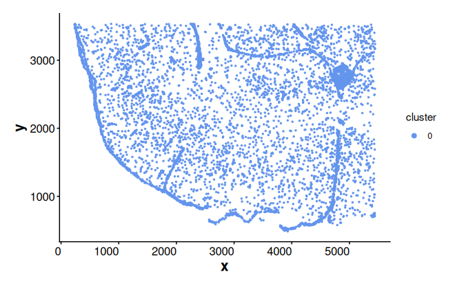

Get boundaries of cluster 0

bon_points_c0 <- getBoundary(data = coords, one_cluster = 0)
bon_polys_c0 <- buildBoundaryPoly(bon_points_c0)

Plot boundary edges for cluster 0

plotEdge(boundary_poly = bon_polys_c0, linewidth_boundary = 0.6)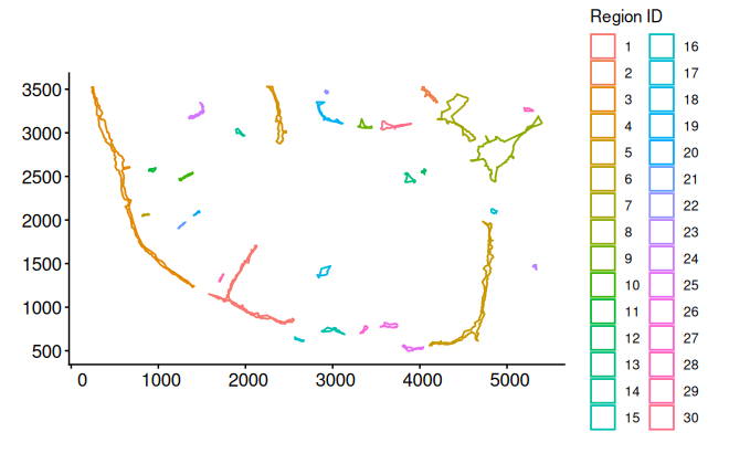

Compute and plot spatial weights

Compute spatial weights based on the distance to boundaries

weights_bon <- computeBoundaryWeights(
    data = coords,
    cell_ids = cells_c0,
    boundary = bon_points_c0
)

Spatial weights are a named vector, where names correspond to cell IDs

weights_bon[1:3]
#>        39        42        75 
#> 0.7016421 0.6955660 0.6805249

Alternatively, compute spatial weights based on the distance to centroids

weights_cen <- computeCentroidWeights(data = coords, cell_ids = cells_c0)

Plot boundary weights

plotWeights(data = coords, weights = weights_bon, point_size = 0.8) +
    labs(title = "Boundary weights")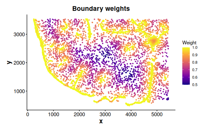

Perform spatial differential analysis along boundary weights

Run spatial DE analysis for cluster 0 cells along boundary weights using splines

tab_sp <- runSpatialDE(
    exp_mat = logNorm_expr[, cells_c0],
    spatial_distance = weights_bon,
    cell_ids = cells_c0
)

Top DE genes along boundary weights. The first spline coefficient (Z1) captures the main expression trend along the spatial distance. A positive value indicates increasing expression with distance, while a negative value indicates decreasing expression.

head(tab_sp)
#>                Z1        Z2        Z3  AveExpr         F P.Value adj.P.Val
#> Aldh1a2  90.19564 -72.83701  18.56803 1.642933 1156.7476       0         0
#> Car4    -86.85851  37.72830 -30.91311 3.007433  590.8437       0         0
#> Col1a1   84.54759 -60.30661  21.47013 1.675953  885.1705       0         0
#> Dcn     112.15109 -72.28618  28.47200 2.337544 1295.7527       0         0
#> Fmod     91.46180 -63.54536  20.99449 1.562370 1083.7186       0         0
#> Gjb2     67.07620 -52.43818  14.55533 1.193263  742.6493       0         0
#>            gene    trend
#> Aldh1a2 Aldh1a2 Positive
#> Car4       Car4 Negative
#> Col1a1   Col1a1 Positive
#> Dcn         Dcn Positive
#> Fmod       Fmod Positive
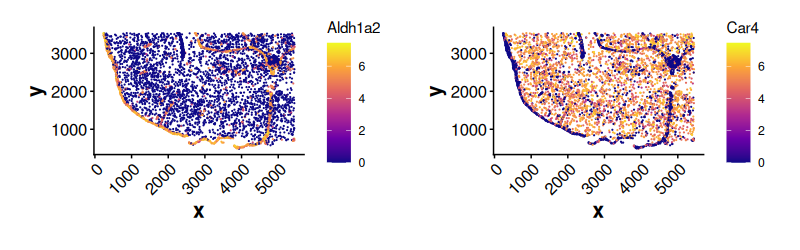
#> Gjb2       Gjb2 Positive

Expression of top DE genes along boundary weights

plotExpression(
    data = coords[colnames(logNorm_expr), ],
    exp_mat = logNorm_expr,
    genes = tab_sp$gene[1:2],
    sub_plot = TRUE,
    one_cluster = 0,
    shuffle = TRUE,
    point_size = 0.1,
    angle_x_label = 45
)

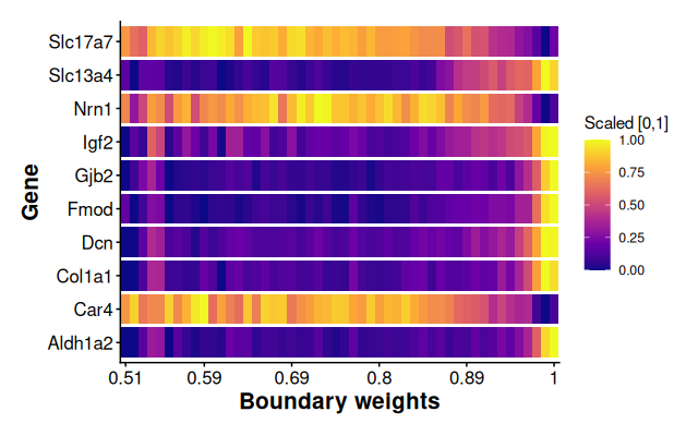
Plot scaled average expression along boundary weight bins for top 10 spatial DE genes. The scaled average expression ranges from 0 to 1 by using min-max normalization method.

plotSpatialExpression(
    exp_mat = logNorm_expr[, cells_c0],
    spatial_distance = weights_bon,
    scale_method = "minmax",
    genes = tab_sp$gene[1:10],
    label_x = "Boundary weights"
)

Spatial enrichment analysis for each gene

Compute spatial enrichment index (SEI) for each gene based on boundary weights. The SEI reflects the extent to which gene expression is enriched in spatially weighted regions. The result is sorted in descending order by normalized_SEI.

SEI_bon <- computeSpatialEnrichmentIndex(
    exp_mat = logNorm_expr[, cells_c0],
    weights = weights_bon
)
head(SEI_bon)
#>      gene      SEI mean_expr normalized_SEI
#> 1    Fmod 1.742086  1.562370       1.115027
#> 2    Gjb2 1.325063  1.193263       1.110452
#> 3 Aldh1a2 1.820161  1.642933       1.107872
#> 4 Slc13a4 2.106610  1.906511       1.104955
#> 5  Col1a1 1.842083  1.675953       1.099125
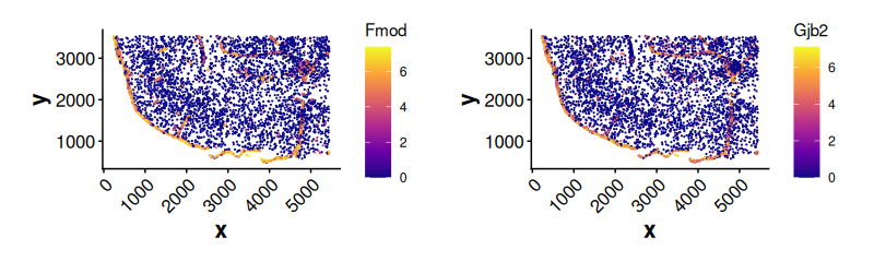
#> 6  Cyp1b1 1.495145  1.365958       1.094575

Expression of top genes enriched near boundaries

plotExpression(
    data = coords[colnames(logNorm_expr), ],
    exp_mat = logNorm_expr,
    genes = SEI_bon$gene[1:2],
    sub_plot = TRUE,
    one_cluster = 0,
    shuffle = TRUE,
    point_size = 0.1,
    angle_x_label = 45
)

Session Info

sessionInfo()
#> R version 4.4.2 (2024-10-31)
#> Platform: x86_64-pc-linux-gnu
#> Running under: Ubuntu 24.04.1 LTS
#> 
#> Matrix products: default
#> BLAS:   /usr/lib/x86_64-linux-gnu/openblas-pthread/libblas.so.3 
#> LAPACK: /usr/lib/x86_64-linux-gnu/openblas-pthread/libopenblasp-r0.3.26.so;  LAPACK version 3.12.0
#> 
#> locale:
#>  [1] LC_CTYPE=en_US.UTF-8       LC_NUMERIC=C              
#>  [3] LC_TIME=en_US.UTF-8        LC_COLLATE=en_US.UTF-8    
#>  [5] LC_MONETARY=en_US.UTF-8    LC_MESSAGES=en_US.UTF-8   
#>  [7] LC_PAPER=en_US.UTF-8       LC_NAME=C                 
#>  [9] LC_ADDRESS=C               LC_TELEPHONE=C            
#> [11] LC_MEASUREMENT=en_US.UTF-8 LC_IDENTIFICATION=C       
#> 
#> time zone: UTC
#> tzcode source: system (glibc)
#> 
#> attached base packages:
#> [1] stats     graphics  grDevices utils     datasets  methods   base     
#> 
#> other attached packages:
#> [1] Seurat_5.4.0       SeuratObject_5.3.0 sp_2.2-1           ggplot2_4.0.2     
#> [5] SpNeigh_0.99.41    BiocStyle_2.34.0  
#> 
#> loaded via a namespace (and not attached):
#>   [1] RcppAnnoy_0.0.23            splines_4.4.2              
#>   [3] later_1.4.6                 tibble_3.3.1               
#>   [5] polyclip_1.10-7             fastDummies_1.7.5          
#>   [7] lifecycle_1.0.5             sf_1.0-24                  
#>   [9] globals_0.19.0              lattice_0.22-9             
#>  [11] MASS_7.3-65                 magrittr_2.0.4             
#>  [13] limma_3.62.2                plotly_4.12.0              
#>  [15] sass_0.4.10                 rmarkdown_2.30             
#>  [17] jquerylib_0.1.4             yaml_2.3.12                
#>  [19] httpuv_1.6.16               otel_0.2.0                 
#>  [21] sctransform_0.4.3           spam_2.11-3                
#>  [23] spatstat.sparse_3.1-0       reticulate_1.45.0          
#>  [25] cowplot_1.2.0               pbapply_1.7-4              
#>  [27] DBI_1.2.3                   RColorBrewer_1.1-3         
#>  [29] abind_1.4-8                 zlibbioc_1.52.0            
#>  [31] Rtsne_0.17                  GenomicRanges_1.58.0       
#>  [33] purrr_1.2.1                 BiocGenerics_0.52.0        
#>  [35] GenomeInfoDbData_1.2.13     IRanges_2.40.1             
#>  [37] S4Vectors_0.44.0            ggrepel_0.9.6              
#>  [39] irlba_2.3.7                 listenv_0.10.0             
#>  [41] spatstat.utils_3.2-1        units_1.0-0                
#>  [43] goftest_1.2-3               RSpectra_0.16-2            
#>  [45] spatstat.random_3.4-4       fitdistrplus_1.2-6         
#>  [47] parallelly_1.46.1           pkgdown_2.2.0              
#>  [49] codetools_0.2-20            DelayedArray_0.32.0        
#>  [51] tidyselect_1.2.1            UCSC.utils_1.2.0           
#>  [53] farver_2.1.2                matrixStats_1.5.0          
#>  [55] stats4_4.4.2                spatstat.explore_3.7-0     
#>  [57] jsonlite_2.0.0              e1071_1.7-17               
#>  [59] progressr_0.18.0            ggridges_0.5.7             
#>  [61] survival_3.8-6              systemfonts_1.3.1          
#>  [63] dbscan_1.2.4                tools_4.4.2                
#>  [65] ragg_1.5.0                  ica_1.0-3                  
#>  [67] Rcpp_1.1.1                  glue_1.8.0                 
#>  [69] gridExtra_2.3               SparseArray_1.6.2          
#>  [71] xfun_0.56                   MatrixGenerics_1.18.1      
#>  [73] GenomeInfoDb_1.42.3         dplyr_1.2.0                
#>  [75] withr_3.0.2                 BiocManager_1.30.27        
#>  [77] fastmap_1.2.0               digest_0.6.39              
#>  [79] R6_2.6.1                    mime_0.13                  
#>  [81] textshaping_1.0.4           scattermore_1.2            
#>  [83] tensor_1.5.1                spatstat.data_3.1-9        
#>  [85] tidyr_1.3.2                 generics_0.1.4             
#>  [87] data.table_1.18.2.1         FNN_1.1.4.1                
#>  [89] class_7.3-23                httr_1.4.8                 
#>  [91] htmlwidgets_1.6.4           S4Arrays_1.6.0             
#>  [93] uwot_0.2.4                  pkgconfig_2.0.3            
#>  [95] gtable_0.3.6                lmtest_0.9-40              
#>  [97] S7_0.2.1                    SingleCellExperiment_1.28.1
#>  [99] XVector_0.46.0              htmltools_0.5.9            
#> [101] dotCall64_1.2               bookdown_0.46              
#> [103] scales_1.4.0                Biobase_2.66.0             
#> [105] png_0.1-8                   SpatialExperiment_1.16.0   
#> [107] spatstat.univar_3.1-6       knitr_1.51                 
#> [109] reshape2_1.4.5              rjson_0.2.23               
#> [111] nlme_3.1-168                curl_7.0.0                 
#> [113] proxy_0.4-29                cachem_1.1.0               
#> [115] zoo_1.8-15                  stringr_1.6.0              
#> [117] KernSmooth_2.23-26          parallel_4.4.2             
#> [119] miniUI_0.1.2                concaveman_1.2.0           
#> [121] desc_1.4.3                  pillar_1.11.1              
#> [123] grid_4.4.2                  vctrs_0.7.1                
#> [125] RANN_2.6.2                  promises_1.5.0             
#> [127] xtable_1.8-4                cluster_2.1.8.2            
#> [129] evaluate_1.0.5              magick_2.9.0               
#> [131] cli_3.6.5                   compiler_4.4.2             
#> [133] rlang_1.1.7                 crayon_1.5.3               
#> [135] future.apply_1.20.1         labeling_0.4.3             
#> [137] classInt_0.4-11             plyr_1.8.9                 
#> [139] fs_1.6.6                    stringi_1.8.7              
#> [141] viridisLite_0.4.3           deldir_2.0-4               
#> [143] lazyeval_0.2.2              spatstat.geom_3.7-0        
#> [145] V8_8.0.1                    Matrix_1.7-4               
#> [147] RcppHNSW_0.6.0              patchwork_1.3.2            
#> [149] future_1.69.0               statmod_1.5.1              
#> [151] shiny_1.12.1                SummarizedExperiment_1.36.0
#> [153] ROCR_1.0-12                 igraph_2.2.2               
#> [155] bslib_0.10.0

Jinming Cheng

17 February, 2026

Introduction

Overview of this vignette

Installation

Load packages

Load data

Input: Coordinate data frame and Normalized expression matrix

Alternative input: SpatialExperiment object

Alternative input: Seurat object

Neighborhood analysis for cluster 2 cells

Quick look at the boundaries of one cluster

Detect spatial boundaries

Obtain neighborhood ring regions

Statistics of cells inside rings

Neighborhood interaction of clusters inside rings

DE analysis of cluster 2 cells inside and outside boundaries

Spatial DE analysis of cells in cluster 0 along spatial weights

Detect spatial boundaries

Compute and plot spatial weights

Perform spatial differential analysis along boundary weights

Spatial enrichment analysis for each gene

Session Info